Overview
This project will cover the following topics:
1. Second Order inverse differential kinematics of a Scara robotic Arm
2. Obstacle Avoidance by maximizing distance between joins and an Obstacle
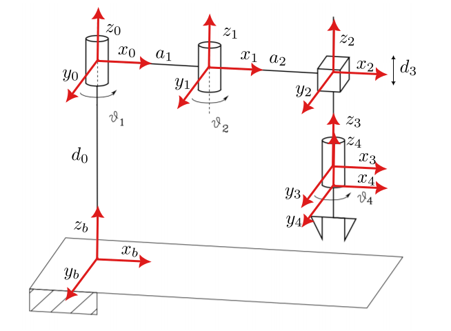
Consider the SCARA manipulator depicted below.
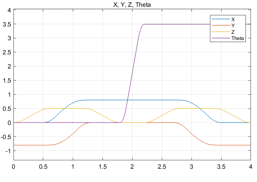
Our Goal is to have the SCARA manipulator end effector follow the given position and velocity trajectories.
Implement in Matlab/Simulink a second order algorithm for kinematic inversion with jacobian inverse along the given trajectory. Adopt the Euler integration rule with integration time 1 ms.
Given trajectory
Our Goal is to have the SCARA manipulator end effector follow the given position and velocity trajectories.
Implement in Matlab/Simulink a second order algorithm for kinematic inversion with jacobian inverse along the given trajectory. Adopt the Euler integration rule with integration time 1 ms.
Second Order Inverse Kinematics using Jacobian Inverse
The Second order inverse kinematics equation for the given manipulator is given by
\[ \ddot{q} = J^{-1}_a(q)(\ddot{x}_d + K_d\dot{e}+K_pe-\dot{J_a}(q,\dot{q})\dot{q})\]
Where \(J^{-1}_a(q)\) is the inverse of the Jacobian. \(\ddot{x_d}\) is the acceleration trajectory. \(e\) is the error between the given trajectory and the end effector position. \(K_d\) and \(K_p\) are gains. For the SCARA robot the Jacobian is a 4×4 matrix. Since the \(Z\) component of the end effector is parallel to the \(Z\) component of the base frame the Geometric Jacobian is equal to the Analytical Jacobian.
The equation given above is modeled using the following kinematic control schematic diagram.
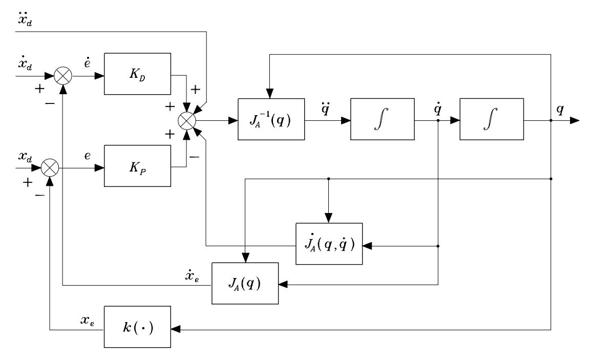
Simulink Block Diagram
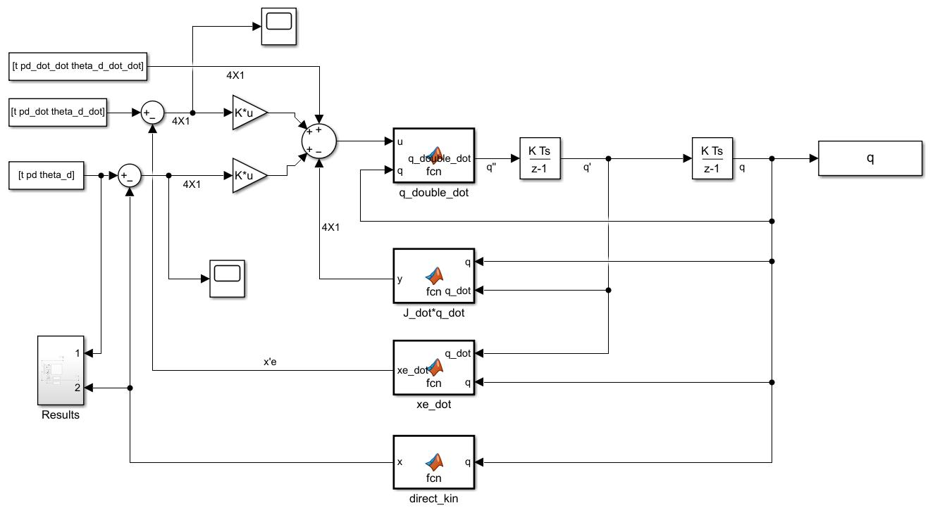
The time series trajectory data is imported from the workspace. A subtract block is used to calculate the error between the required trajectory and the actual position of the end effector which is calculated using direct kinematics. The error signal is passed through a gain block.
\(J_a(q,\dot{q})\) is calculated by differentiating \(J_a(q)\) with respect to \(t\).
\[\frac{dJ_a}{dt} =\frac{dJ_a}{dq}∙\frac{dq}{dt}\]
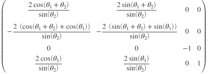
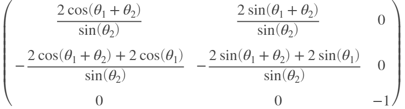
We get \(J_a(q)\) as

Finally the function “q_double_dot” is used to bring together all the terms and calculate \[\ddot{q} = J^{-1}_a(q)(\ddot{x_d}+K_d\dot{e}+K_pe-\dot{J_a}(q,\dot{q})\dot{q})\]
Here \(J_a^{-1}(q)\) is found to be
\(\ddot{q}\) is integrated twice to get \(q\). The mechanical joint limits are entered in the discrete integrator block . The upper saturation limit is \([π/2, \: π/4, \: 1, \: 2π]^T\) and the lower saturation limit is \([−π/2, \: −π/2, \: 1/4, \: −2π]^T\).
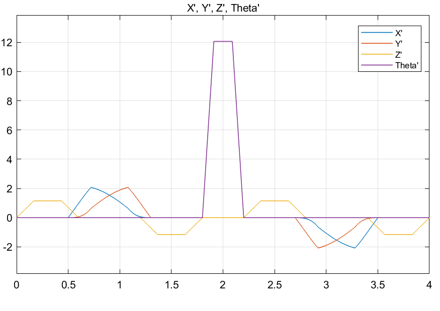
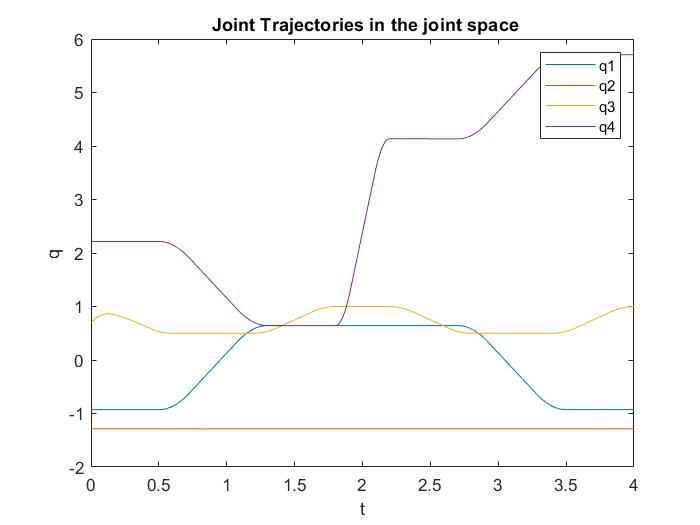
Results
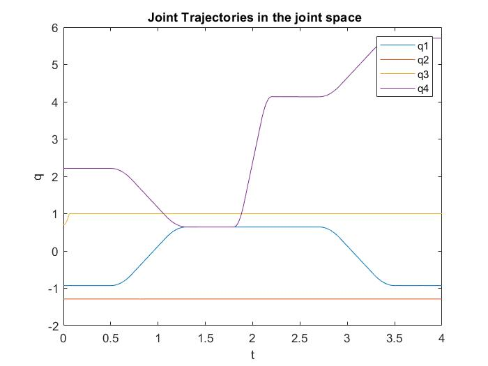
Joint space trajectories are found to be.
Part 2
Suppose to relax one component in the operational space (relax the z component), implement in Matlab/Simulink the second order algorithm for kinematic inversion with Jacobian pseudo-inverse along the given trajectory maximizing the distance from an obstacle along the path. Suppose that the obstacle is a sphere centered in p = [0.4 −0.7 0.5]⊤ with radius 0.2 m.
Exploit Redundancy using Jacobian Pseudo-inverse
\[ \ddot{q} = J^{+}_a(\ddot{x}_d + K_d\dot{e}+K_pe-\dot{J_a}(q,\dot{q})\dot{q})+(I_n-J^{+}_aJ_a)\ddot{q}_0 \]
Where \(J^{+}_a\) is the Jacobian Pseudo inverse.
\(\dot{q}_0\) enables us to generate internal motions and optimize for certain criteria without changing end effector position. In our case we want to stay as close as possible to the center of the joint range.
\[\dot{q}_0 = k_0 \left( \frac{\partial w(q)}{\partial q} \right)^T\]
where \(k_0 > 0\) and \(w(q)\) is a (secondary) objective function of the joint variables.
\[w(q)= _{p, o}^{min} ||p(q)−o||\]
Here \(w(q)\) is a cost function that when minimized ensures that the end distance between the effector position pq and the obstacle \((o)\) is maximized.
The distance is calculated using the equation
\[w(q) = \sqrt{(p_x−o_x)^2+(p_y−o_y)^2+(p_z−o_z)^2}\]
Substituting \(p_x, p_y\) and \(p_z\) \[ \sqrt{\left( \frac{cos(\theta_1+\theta_2)}{2} + \frac{cos(\theta_1)}{2}-\frac{2}{5} \right)^2 + \left( \frac{sin(\theta_1+\theta_2)}{2} + \frac{sin(\theta_1)}{2}-\frac{7}{10} \right)^2 + \left( d_3 - \frac{1}{2} \right) }\]
Integrating twice with respect to “q” and multiply gain ‘\(k_0\)’ we get \(q_0\).
Simulink Block Diagram
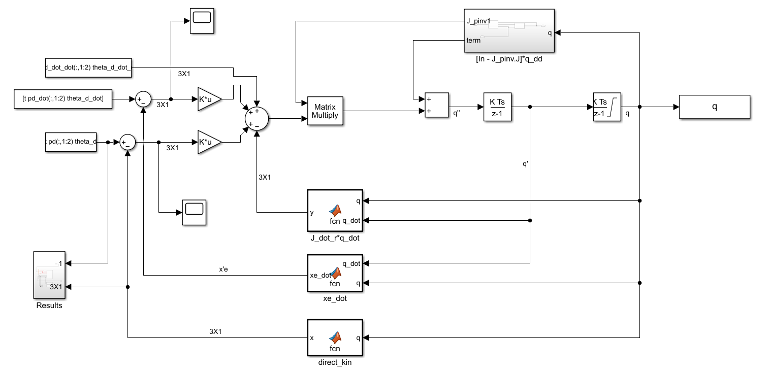
The Simulink Network above is very similar to the previous block diagrams. However it has a few key differences.
Firstly, the ‘\(Z\)’ term has been relaxed. Hence it is not input into the system. The direct_kin, xe_dot and J_dot_r*q_dot block is the same as that implemented in previous model. However,the code has been altered to accommodate the relaxed Jacobian. In essence, converting a 4×1 matrix to a 3×1 matrix.
Secondly I have implemented the subsystem “[In - J_pinv.J]*q_dd”. Subsystem one takes input ‘q’ and returns the jacobian pseudo inverse ‘J_pinv’ and an additional term In− JA†JAq0.
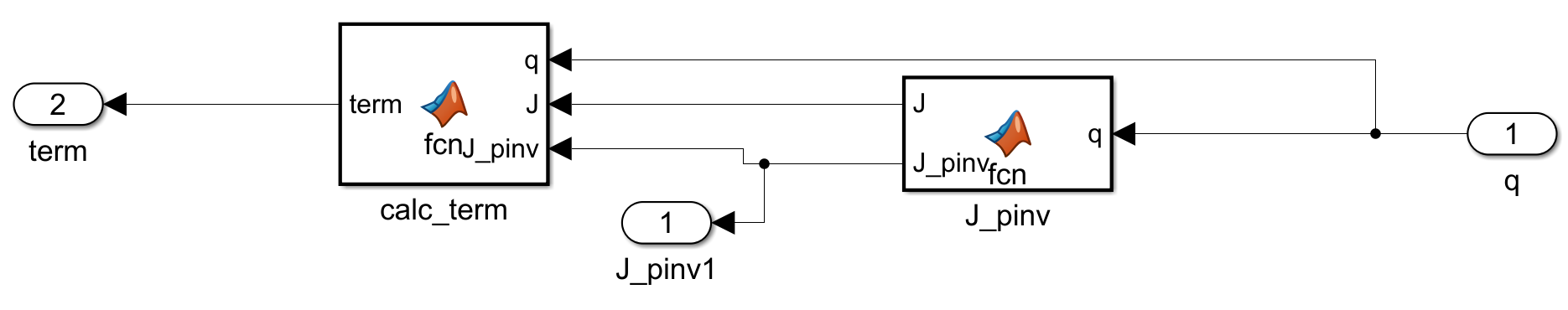
“[In - J_pinv.J]*q_dd” Subsystem
The subsystem is composed of two functions. The “J_pinv” function takes as input “q” and returns the Jacobian “J” and the Jacobian pseudo-inverse “J_pinv”. The function “calc_term” returns the term \((I_n− J_a^†J_a)\ddot{q_0}\)
Results
Joint space trajectories are found to be. Notice that q3 is constant this correlates with the lowest position of the end effector. In essence, the maximum distance from the obstacle.
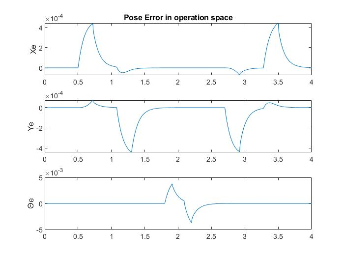
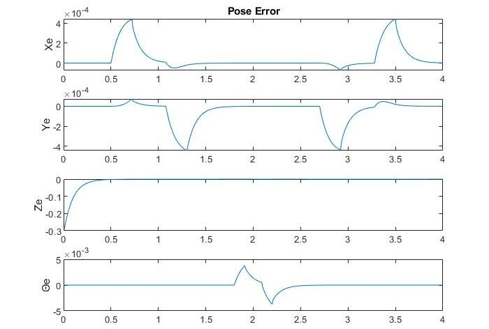
The error vs time chart for the end effector positions along X,Y and Θ axes are given.